 |
 |
|
||||
|
By
Wikipedia,
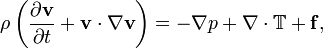
The Navier–Stokes equations, named after Claude-Louis Navier and George Gabriel Stokes, describe the motion of fluid substances, that is substances which can flow. These equations arise from applying Newton's second law to fluid motion, together with the assumption that the fluid stress is the sum of a diffusing viscous term (proportional to the gradient of velocity), plus a pressure term. They are one of the most useful sets of equations because they describe the physics of a large number of phenomena of academic and economic interest. They may be used to model weather, ocean currents, water flow in a pipe, flow around an airfoil (wing), and motion of stars inside a galaxy. As such, these equations in both full and simplified forms, are used in the design of aircraft and cars, the study of blood flow, the design of power stations, the analysis of the effects of pollution, etc. Coupled with Maxwell's equations they can be used to model and study magnetohydrodynamics. The Navier–Stokes equations are also of great interest in a purely mathematical sense. Somewhat surprisingly, given their wide range of practical uses, mathematicians have not yet proven that in three dimensions solutions always exist (existence), or that if they do exist they do not contain any infinities, singularities or discontinuities (smoothness). These are called the Navier–Stokes existence and smoothness problems. The Clay Mathematics Institute has called this one of the seven most important open problems in mathematics, and offered a US$1,000,000 prize for a solution or a counter-example. The Navier–Stokes equations are differential equations which, unlike algebraic equations, do not explicitly establish a relation among the variables of interest (e.g. velocity and pressure). Rather, they establish relations among the rates of change. For example, the Navier–Stokes equations for simple case of an ideal fluid (inviscid and incompressible) can state that acceleration (the rate of change of velocity) is proportional to the gradient (a type of multivariate derivative) of pressure. The Navier–Stokes equations dictate not position but rather velocity. A solution of the Navier–Stokes equations is called a velocity field or flow field, which is a description of the velocity of the fluid at a given point in space and time. Once the velocity field is solved for, other quantities of interest (such as flow rate or drag force) may be found. This is different from what one normally sees in classical mechanics, where solutions are typically trajectories of position of a particle or deflection of a continuum. Studying velocity instead of position makes more sense for a fluid, however for visualization purposes one can compute various trajectories. PropertiesNonlinearityThe Navier–Stokes equations are nonlinear partial differential equations in almost every real situation. In some cases, such as one-dimensional flow and Stokes flow (or creeping flow), the equations can be simplified to linear equations. The nonlinearity makes most problems difficult or impossible to solve and is the main contributor to the turbulence that the equations model. The nonlinearity is due to convective acceleration, which is an acceleration associated with the change in velocity over position. Hence, any convective flow, whether turbulent or not, will involve nonlinearity, an example of convective but laminar (nonturbulent) flow would be the passage of a viscous fluid (for example, oil) through a small converging nozzle. Such flows, whether exactly solvable or not, can often be thoroughly studied and understood. TurbulenceTurbulence is the time dependent chaotic behavior seen in many fluid flows. It is generally believed that it is due to the inertia of the fluid as a whole: the culmination of time dependent and convective acceleration; hence flows where inertial effects are small tend to be laminar (the Reynolds number quantifies how much the flow is affected by inertia). It is believed, though not known with certainty, that the Navier–Stokes equations describe turbulence properly. The numerical solution of the Navier–Stokes equations for turbulent flow is extremely difficult, and due to the significantly different mixing-length scales that are involved in turbulent flow, the stable solution of this requires such a fine mesh resolution that the computational time becomes significantly infeasible for calculation (see Direct numerical simulation). Attempts to solve turbulent flow using a laminar solver typically result in a time-unsteady solution, which fails to converge appropriately. To counter this, time-averaged equations such as the Reynolds-averaged Navier-Stokes equations (RANS), supplemented with turbulence models (such as the k-ε model), are used in practical computational fluid dynamics (CFD) applications when modeling turbulent flows. Another technique for solving numerically the Navier–Stokes equation is the Large-eddy simulation (LES). This approach is computationally more expensive than the RANS method (in time and computer memory), but produces better results since the larger turbulent scales are explicitly resolved. ApplicabilityTogether with supplemental equations (for example, conservation of mass) and well formulated boundary conditions, the Navier–Stokes equations seem to model fluid motion accurately; even turbulent flows seem (on average) to agree with real world observations. The Navier–Stokes equations assume that the fluid being studied is a continuum not moving at relativistic velocities. At very small scales or under extreme conditions, real fluids made out of discrete molecules will produce results different from the continuous fluids modeled by the Navier–Stokes equations. Depending on the Knudsen number of the problem, statistical mechanics or possibly even molecular dynamics may be a more appropriate approach. Another limitation is very simply the complicated nature of the equations. Time tested formulations exist for common fluid families, but the application of the Navier–Stokes equations to less common families tends to result in very complicated formulations which are an area of current research. For this reason, the Navier–Stokes equations are usually written for Newtonian fluids. Almost universally the equations are written for a simple class of fluids (which most liquids and all known gases belong to) known as Newtonian fluids. Studying such fluids is "simple" because the viscosity model ends up being linear; truly general models for the flow of other kinds of fluids (such as blood) do not, as of 2009, exist. Derivation and descriptionThe derivation of the Navier–Stokes equations begins with an application of Newton's second law: conservation of momentum (often alongside mass and energy conservation) being written for an arbitrary control volume. In an inertial frame of reference, the general form of the equations of fluid motion is: where This equation is often written using the substantive derivative, making it more apparent that this is a statement of Newton's second law: The left side of the equation describes acceleration, and may be composed of time dependent or convective effects (also the effects of non-inertial coordinates if present). The right side of the equation is in effect a summation of body forces (such as gravity) and divergence of stress (pressure and stress). Convective acceleration
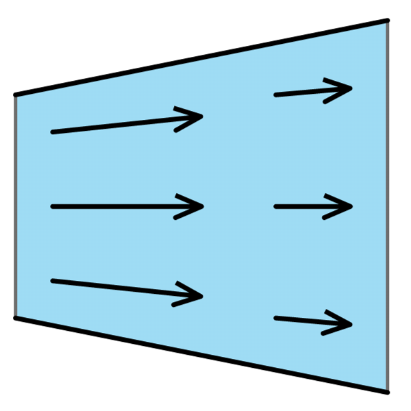
A very significant feature of the Navier–Stokes equations is the presence of convective acceleration: the effect of time independent acceleration of a fluid with respect to space, represented by the nonlinear quantity: which may be interpreted either as Interpretation as (v·∇)vThe convection term is often written as where the advection operator Interpretation as v·(∇v)Here The form has use in irrotational flow, where the curl of the velocity (called vorticity) Regardless of what kind of fluid is being dealt with, convective acceleration is a nonlinear effect. Convective acceleration is present in most flows (exceptions include one-dimensional incompressible flow), but it's dynamic effect is disregarded in creeping flow (also called Stokes flow) . StressesThe effect of stress in the fluid is represented by the where The stress terms p and The pressure p is modelled by use of an equation of state. For the special case of an incompressible flow, the pressure constrains the flow in such a way that the volume of fluid elements is constant: isochoric flow resulting in a solenoidal velocity field with Other forcesThe vector field Often, these forces may be represented as the gradient of some scalar quantity. Gravity in the z direction, for example, is the gradient of − ρgz. Since pressure shows up only as a gradient, this implies that solving a problem without any such body force can be mended to include the body force by modifying pressure. Other equationsThe Navier–Stokes equations are strictly a statement of the conservation of momentum. In order to fully describe fluid flow, more information is needed (how much depends on the assumptions made), this may include boundary data (no-slip, capillary surface, etc), the conservation of mass, the conservation of energy, and/or an equation of state. Regardless of the flow assumptions, a statement of the conservation of mass is generally necessary. This is achieved through the mass continuity equation, given in its most general form as: or, using the substantive derivative: Incompressible flow of Newtonian fluidsA simplification of the resulting flow equations is obtained when considering an incompressible flow of a Newtonian fluid. The assumption of incompressibility rules out the possibility of sound or shock waves to occur; so this simplification is invalid if these phenomena are important. The incompressible flow assumption typically holds well even when dealing with a "compressible" fluid — such as air at room temperature — at low Mach numbers (even when flowing up to about Mach 0.3). Taking the incompressible flow assumption into account and assuming constant viscosity, the Navier–Stokes equations will read, in vector form: Here f represents "other" body forces (forces per unit volume), such as gravity or centrifugal force. The shear stress term
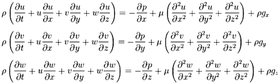
Note that only the convective terms are nonlinear for incompressible Newtonian flow. The convective acceleration is an acceleration caused by a (possibly steady) change in velocity over position, for example the speeding up of fluid entering a converging nozzle. Though individual fluid particles are being accelerated and thus are under unsteady motion, the flow field (a velocity distribution) will not necessarily be time dependent. Another important observation is that the viscosity is represented by the vector Laplacian of the velocity field. This implies that Newtonian viscosity is diffusion of momentum, this works in much the same way as the diffusion of heat seen in the heat equation (which also involves the Laplacian). If temperature effects are also neglected, the only "other" equation (apart from initial/boundary conditions) needed is the mass continuity equation. Under the incompressible assumption, density is a constant and it follows that the equation will simplify to: This is more specifically a statement of the conservation of volume (see divergence). These equations are commonly used in 3 coordinates systems: Cartesian, cylindrical, and spherical. While the Cartesian equations seem to follow directly from the vector equation above, the vector form of the Navier–Stokes equation involves some tensor calculus which means that writing it in other coordinate systems is not as simple as doing so for scalar equations (such as the heat equation). Cartesian coordinatesWriting the vector equation explicitly,
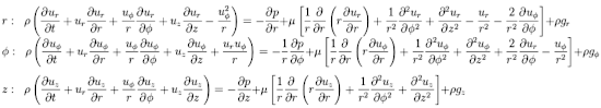
Note that gravity has been accounted for as a body force, and the values of gx,gy,gz will depend on the orientation of gravity with respect to the chosen set of coordinates. The continuity equation reads: The velocity components (the dependent variables to be solved for) are typically named u, v, w. This system of four equations comprises the most commonly used and studied form. Though comparatively more compact than other representations, this is a nonlinear system of partial differential equations for which solutions are difficult to obtain. Cylindrical coordinatesA change of variables on the Cartesian equations will yield the following momentum equations for r, φ, and z:
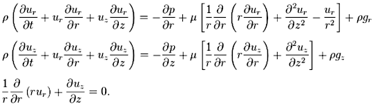
The gravity components will generally not be constants, however for most applications either the coordinates are chosen so that the gravity components are constant or else it is assumed that gravity is counteracted by a pressure field (for example, flow in horizontal pipe is treated normally without gravity and without a vertical pressure gradient). The continuity equation is: This cylindrical representation of the incompressible Navier–Stokes equations is the second most commonly seen (the first being Cartesian above). Cylindrical coordinates are chosen to take advantage of symmetry, so that a velocity component can disappear. A very common case is axisymmetric flow with the assumption of no tangential velocity (uφ = 0), and the remaining quantities are independent of φ:
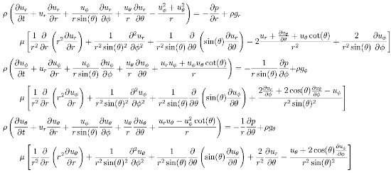
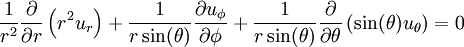
Spherical coordinatesIn spherical coordinates, the r, θ, and φ momentum equations are (note the convention used: θ is colatitude):
Mass continuity will read: These equations could be (slightly) compacted by, for example, factoring 1 / r from the viscous terms. This isn't done to preserve the structure of the Laplacian and other quantities. Stream function formulationTaking the curl of the Navier–Stokes equation results in the elimination of pressure. This is especially easy to see if 2D Cartesian flow is assumed (w = 0 and no dependence of anything on z), where the equations reduce to:
Differentiating the first with respect to y, the second with respect to x and subtracting the resulting equations will eliminate pressure and any potential force. Defining the stream function ψ through
results in mass continuity being unconditionally satisfied (given the stream function is continuous), and then incompressible Newtonian 2D momentum and mass conservation degrade into one equation:
where In axisymmetric flow another stream function formulation, called the Stokes stream function, can be used to describe the velocity components of an incompressible flow with one scalar function. Compressible flow of Newtonian fluidsThere are some phenomena that are closely linked with fluid compressibility. One of the obvious examples is sound. Description of such phenomena requires more general presentation of the Navier–Stokes equation that takes into account fluid compressibility. If viscosity is assumed a constant, one additional term appears, as shown here:
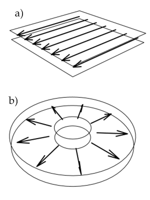
where μ is second viscosity coefficient. It is related to volume viscosity or bulk viscosity. This additional term disappears for incompressible fluid, when the divergence of the flow equals zero. Application to specific problemsThe Navier–Stokes equations, even when written explicitly for specific fluids, are rather generic in nature and their proper application to specific problems can be very diverse. This is partly because there is an enormous variety of problems that may be modeled, ranging from as simple as the distribution of static pressure to as complicated as multiphase flow driven by surface tension. Generally, application to specific problems begins with some flow assumptions and initial/boundary condition formulation, this may be followed by scale analysis to further simplify the problem. For example, after assuming steady, parallel, one dimensional, nonconvective pressure driven flow between parallel plates, the resulting scaled (dimensionless) boundary value problem is:
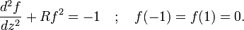
The boundary condition is the no slip condition. This problem is easily solved for the flow field: From this point onward more quantities of interest can be easily obtained, such as viscous drag force or net flow rate. Difficulties may arise when the problem becomes slightly more complicated. A seemingly modest twist on the parallel flow above would be the radial flow between parallel plates; this involves convection and thus nonlinearity. The velocity field may be represented by a function f(z) that must satisfy: This ordinary differential equation is what is obtained when the Navier–Stokes equations are written and the flow assumptions applied (additionally, the pressure gradient is solved for). The nonlinear term makes this a very difficult problem to solve analytically (a lengthy implicit solution may be found which involves elliptic integrals and roots of cubic polynomials). Issues with the actual existence of solutions arise for R > 1.41 (approximately. This is not the square root of two), the parameter R being the Reynolds number with appropriately chosen scales. This is an example of flow assumptions losing their applicability, and an example of the difficulty in "high" Reynolds number flows. Exact solutions of the Navier–Stokes equationsSome exact solutions to the Navier–Stokes equations exist. Examples of degenerate cases — with the non-linear terms in the Navier–Stokes equations equal to zero — are Poiseuille flow, Couette flow and the oscillatory Stokes boundary layer. But also more interesting examples, solutions to the full non-linear equations, exist; for example the Taylor–Green vortex. Note that the existence of these exact solutions does not imply they are stable: turbulence may develop at higher Reynolds numbers. Wyld diagramsWyld diagrams are bookkeeping graphs that correspond to the Navier–Stokes equations via a perturbation expansion of the fundamental continuum mechanics. Similar to the Feynman diagrams in quantum field theory (QFT), these diagrams are an extension of Keldysh's technique for nonequilibrium processes in fluid dynamics. In other words, these diagrams assign graphs to (the often) turbulent phenomena in turbulent fluids by allowing correlated and interacting fluid particles to obey stochastic processes associated to pseudo-random functions in probability distributions. See also
Text from Wikipedia is available under the Creative Commons Attribution/Share-Alike License; additional terms may apply.
Published in July 2009. Click here to read more articles related to aviation and space!
|

 |
|
Copyright 2004-2025 © by Airports-Worldwide.com, Vyshenskoho st. 36, Lviv 79010, Ukraine Legal Disclaimer |

 is the flow velocity,
  is the (
 represents
  is the
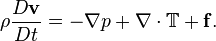

 or as
or as  with
with  the
the  Both interpretations give the same result, independent of the coordinate system — provided
 is used. Usually this representation is preferred because it is simpler than the one in terms of the tensor derivative

 is equal to zero.
 and
and  terms, these are gradients of surface forces, analogous to stresses in a solid.
  is the
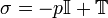
 is the 3×3
 represents "other" (


 becomes the useful quantity
  when the fluid is assumed incompressible and
  is the dynamic viscosity.


 is the (2D)
  . This single equation together with appropriate boundary conditions describes 2D fluid flow, taking only kinematic viscosity as a parameter. Note that the equation for