Orbital mechanics

Orbital mechanics

By Wikipedia,
the free encyclopedia,

https://en.wikipedia.org/wiki/Orbital_mechanics

Orbital mechanics or astrodynamics is the application of celestial mechanics to the practical problems concerning the motion of rockets and other spacecraft. The motion of these objects is usually calculated from Newton's laws of motion and Newton's law of universal gravitation. It is a core discipline within space mission design and control. Celestial mechanics treats more broadly the orbital dynamics of systems under the influence of gravity, including both spacecraft and natural astronomical bodies such as star systems, planets, moons, and comets. Orbital mechanics focuses on spacecraft trajectories, including orbital maneuvers, orbit plane changes, and interplanetary transfers, and is used by mission planners to predict the results of propulsive maneuvers. General relativity is a more exact theory than Newton's laws for calculating orbits, and is sometimes necessary for greater accuracy or in high-gravity situations (such as orbits close to the Sun).

A satellite orbiting the earth has a tangential velocity and an inward acceleration.

A satellite orbiting the earth has a tangential velocity and an inward acceleration.

Rules of thumb

The following rules of thumb are useful for situations approximated by classical mechanics under the standard assumptions of astrodynamics. The specific example discussed is of a satellite orbiting a planet, but the rules of thumb could also apply to other situations, such as orbits of small bodies around a star such as the Sun.

Kepler's laws of planetary motion, which can be mathematically derived from Newton's laws, hold strictly only in describing the motion of two gravitating bodies, in the absence of non-gravitational forces, or approximately when the gravity of a single massive body like the Sun dominates other effects:
- Orbits are either circular, with the planet at the center of the circle, or elliptical, with the planet at one focus of the ellipse.
- A line drawn from the planet to the satellite sweeps out equal areas in equal times no matter which portion of the orbit is measured.
- The square of a satellite's orbital period is proportional to the cube of its average distance from the planet.
Without firing a rocket engine (generating thrust), the height and shape of the satellite's orbit won't change, and it will maintain the same orientation with respect to the fixed stars.
A satellite in a low orbit (or low part of an elliptical orbit) moves more quickly with respect to the surface of the planet than a satellite in a higher orbit (or a high part of an elliptical orbit), due to the stronger gravitational attraction closer to the planet.
If a brief rocket firing is made at only one point in the satellite's orbit, it will return to that same point on each subsequent orbit, though the rest of its path will change. Thus to move from one circular orbit to another, at least two brief firings are needed.
From a circular orbit, a brief firing of a rocket in the direction which slows the satellite down, will create an elliptical orbit with a lower perigee (lowest orbital point) at 180 degrees away from the firing point, which will be the apogee (highest orbital point). If the rocket is fired to speed the rocket, it will create an elliptical orbit with a higher apogee 180 degrees away from the firing point (which will become the perigee).

The consequences of the rules of orbital mechanics are sometimes counter-intuitive. For example, if two spacecraft are in the same circular orbit and wish to dock, unless they are very close, the trailing craft cannot simply fire its engines to go faster. This will change the shape of its orbit, causing it to gain altitude and miss its target. One approach is to actually fire a reverse thrust to slow down, and then fire again to re-circularize the orbit at a lower altitude. Because lower orbits are faster than higher orbits, the trailing craft will begin to catch up. A third firing at the right time will put the trailing craft in an elliptical orbit which will intersect the path of the leading craft, approaching from below.

To the degree that the standard assumptions of astrodynamics do not hold, actual trajectories will vary from those calculated. For example, simple atmospheric drag is another complicating factor for objects in Earth orbit. These rules of thumb are decidedly inaccurate when describing two or more bodies of similar mass, such as a binary star system. (Celestial mechanics uses more general rules applicable to a wider variety of situations.) The differences between classical mechanics and general relativity can also become important for large objects like planets.

History

Until the rise of space travel in the twentieth century, there was little distinction between orbital and celestial mechanics. The fundamental techniques, such as those used to solve the Keplerian problem (determining position as a function of time), are therefore the same in both fields. Furthermore, the history of the fields is almost entirely shared.

Johannes Kepler was the first to successfully model planetary orbits to a high degree of accuracy, publishing his laws in 1605. Isaac Newton published more general laws of celestial motion in his 1687 book, Philosophiæ Naturalis Principia Mathematica.

Practical techniques

Transfer orbits

Transfer orbits allow spacecraft to move from one orbit to another. Usually they require a burn at the start, a burn at the end, and sometimes one or more burns in the middle. The Hohmann transfer orbit typically requires the least delta-v, but any orbit that intersects both the origin orbit and destination orbit may be used.

Gravity assist and the Oberth effect

In a gravity assist, a spacecraft swings by a planet and leaves in a different direction, at a different velocity. This is useful to speed or slow a spacecraft instead of carrying more fuel.

This maneuver can be approximated by an elastic collision at large distances, though the flyby does not involve any physical contact. Due to Newton's Third Law (equal and opposite reaction), any momentum gained by a spacecraft must be lost by the planet, or vice versa. However, because the planet is much, much more massive than the spacecraft, the effect on the planet's orbit is negligible.

The Oberth effect can be employed, particularly during a gravity assist operation. This effect is that use of a propulsion system works better at high speeds, and hence course changes are best done when close to a gravitating body; this can multiply the effective delta-v.

Interplanetary Transport Network and fuzzy orbits

It is now possible to use computers to search for routes using the nonlinearities in the gravity of the planets and moons of the solar system. For example, it is possible to plot an orbit from high earth orbit to Mars, passing close to one of the Earth's Trojan points. Collectively referred to as the Interplanetary Transport Network, these highly perturbative, even chaotic, orbital trajectories in principle need no fuel (in practice keeping to the trajectory requires some course corrections). The biggest problem with them is they can be exceedingly slow, taking many years to arrive. In addition launch windows can be very far apart.

They have, however, been employed on projects such as Genesis. This spacecraft visited Earth's Lagrange L1 point and returned using very little propellant.

Laws of astrodynamics

The fundamental laws of astrodynamics are Newton's law of universal gravitation and Newton's laws of motion, while the fundamental mathematical tool is his differential calculus.

Standard assumptions in astrodynamics include non-interference from outside bodies, negligible mass for one of the bodies, and negligible other forces (such as from the solar wind, atmospheric drag, etc.). More accurate calculations can be made without these simplifying assumptions, but they are more complicated. The increased accuracy often does not make enough of a difference in the calculation to be worthwhile.

Kepler's laws of planetary motion may be derived from Newton's laws, when it is assumed that the orbiting body is subject only to the gravitational force of the central attractor. When an engine thrust or propulsive force is present, Newton's laws still apply, but Kepler's laws are invalidated. When the thrust stops, the resulting orbit will be different but will once again be described by Kepler's laws. The three laws are:

The orbit of every planet is an ellipse with the sun at one of the foci.
A line joining a planet and the sun sweeps out equal areas during equal intervals of time.
The squares of the orbital periods of planets are directly proportional to the cubes of the semi-major axis of the orbits.

Escape velocity

The formula for escape velocity is easily derived as follows. The specific energy (energy per unit mass) of any space vehicle is composed of two components, the specific potential energy and the specific kinetic energy. The specific potential energy associated with a planet of mass M is given by

$- G M / r \,$

while the specific kinetic energy of an object is given by

$v^2/2 \,$

Since energy is conserved, the total specific orbital energy

$v^2/2 - G M / r \,$

does not depend on the distance, $r$ , from the center of the central body to the space vehicle in question. Therefore, the object can reach infinite $r$ only if this quantity is nonnegative, which implies

$v\geq\sqrt{2 G M / r}$

The escape velocity from the Earth's surface is about 11 km/s, but that is insufficient to send the body an infinite distance because of the gravitational pull of the Sun. To escape the solar system from the vicinity of the Earth requires around 42 km/s velocity, but there will be "part credit" for the Earth's orbital velocity for spacecraft launched from Earth, if their further acceleration (due to the propulsion system) carries them in the same direction as Earth travels in its orbit.

Formulae for free orbits

Orbits are conic sections, so, naturally, the formula for the distance of a body for a given angle corresponds to the formula for that curve in polar coordinates, which is:

$r = {p \over (1 + e \cos \theta) }$ .

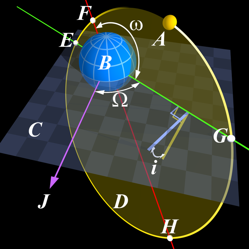
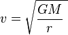
The parameter θ is known as the true anomaly, p is the semi-latus rectum, while e is the eccentricity, all obtainable from the various forms of the six independent orbital elements.

Circular orbits

Although most orbits are elliptical in nature, a special case is the circular orbit, which is an ellipse of zero eccentricity. The formula for the velocity of a body in a circular orbit at distance r from the center of gravity of mass M is

$\ v = \sqrt{\frac{GM} {r}\ }$

where $G$ is the gravitational constant, equal to

6.672 598 × 10 m/(kg·s)

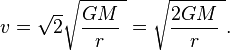
To properly use this formula, the units must be consistent; for example, M must be in kilograms, and r must be in meters. The answer will be in meters per second.

The quantity GM is often termed the standard gravitational parameter, which has a different value for every planet or moon in the solar system.

Once the circular orbital velocity is known, the escape velocity is easily found by multiplying by the square root of 2:

$\ v = \sqrt 2\sqrt{\frac {GM} {r}\ } = \sqrt{\frac {2GM} {r}\ }.$

Mathematical techniques

Kepler's equation

One approach to calculating orbits (mainly used historically) is to use Kepler's equation:

$M=E-e\cdot\sin E$ .

where M is the mean anomaly, E is the eccentric anomaly, and $e$ is eccentricity.

With Kepler's formula, finding the time-of-flight to reach an angle (true anomaly) of $θ$ from periapsis is broken into two steps:

Compute the eccentric anomaly $E$ from true anomaly $θ$
Compute the time-of-flight $t$ from the eccentric anomaly $E$

Finding the angle at a given time is harder. Kepler's equation is transcendental in $E$ , meaning it cannot be solved for $E$ analytically, and so numerical approaches must be used. In effect, one must guess a value of $E$ and solve for time-of-flight; then adjust $E$ as necessary to bring the computed time-of-flight closer to the desired value until the required precision is achieved. Usually, Newton's method is used to achieve relatively fast convergence.

The main difficulty with this approach is that it can take prohibitively long to converge for the extreme elliptical orbits. For near-parabolic orbits, eccentricity $e$ is nearly 1, and plugging $e = 1$ into the formula for mean anomaly, $E - sin E$ , we find ourselves subtracting two nearly-equal values, and so accuracy suffers. For near-circular orbits, it is hard to find the periapsis in the first place (and truly circular orbits have no periapsis at all). Furthermore, the equation was derived on the assumption of an elliptical orbit, and so it does not hold for parabolic or hyperbolic orbits at all. These difficulties are what led to the development of the universal variable formulation, described below.

Perturbation theory

One can deal with perturbations just by summing the forces and integrating, but that is not always best. Historically, variation of parameters has been used which is easier to mathematically apply with when perturbations are small.

Conic orbits

For simple procedures, such as computing the delta-v for coplanar transfer ellipses, traditional approaches are fairly effective. Others, such as time-of-flight are far more complicated, especially for near-circular and hyperbolic orbits.

The patched conic approximation

The Hohmann transfer orbit alone is a poor approximation for interplanetary trajectories because it neglects the planets' own gravity. Planetary gravity dominates the behaviour of the spacecraft in the vicinity of a planet and in most cases Hohmann severely overestimates delta-v, and produces highly inaccurate prescriptions for burn timings.

A relatively simple way to get a first-order approximation of delta-v is based on the Patched Conic Approximation technique. One must choose the one dominant gravitating body in each region of space through which the trajectory will pass, and to model only that body's effects in that region. For instance, on a trajectory from the Earth to Mars, one would begin by considering only the Earth's gravity until the trajectory reaches a distance where the Earth's gravity no longer dominates that of the Sun. The spacecraft would be given escape velocity to send it on its way to interplanetary space. Next, one would consider only the Sun's gravity until the trajectory reaches the neighbourhood of Mars. During this stage, the transfer orbit model is appropriate. Finally, only Mars's gravity is considered during the final portion of the trajectory where Mars's gravity dominates the spacecraft's behaviour. The spacecraft would approach Mars on a hyperbolic orbit, and a final retrograde burn would slow the spacecraft enough to be captured by Mars.

The size of the "neighborhoods" (or spheres of influence) vary with radius $r S O I$ :

$r_{SOI} = a_p\left(\frac{m_p}{m_s}\right)^{2/5}$

where $a p$ is the semimajor axis of the planet's orbit relative to the Sun; $m p$ and $m s$ are the masses of the planet and Sun, respectively.

This simplification is sufficient to compute rough estimates of fuel requirements, and rough time-of-flight estimates, but it is not generally accurate enough to guide a spacecraft to its destination. For that, numerical methods are required.

The universal variable formulation

To address the shortcomings of the traditional approaches, the universal variable formulation was developed. It works equally well on circular, elliptical, parabolic, and hyperbolic orbits; and also works well with perturbation theory. The differential equations converge nicely when integrated for any orbit.

Perturbations

The universal variable formulation works well with the variation of parameters technique, except now, instead of the six Keplerian orbital elements, we use a different set of orbital elements: namely, the satellite's initial position and velocity vectors $x 0$ and $v 0$ at a given epoch $t = 0$ . In a two-body simulation, these elements are sufficient to compute the satellite's position and velocity at any time in the future, using the universal variable formulation. Conversely, at any moment in the satellite's orbit, we can measure its position and velocity, and then use the universal variable approach to determine what its initial position and velocity would have been at the epoch. In perfect two-body motion, these orbital elements would be invariant (just like the Keplerian elements would be).

However, perturbations cause the orbital elements to change over time. Hence, we write the position element as $x 0 (t)$ and the velocity element as $v 0 (t)$ , indicating that they vary with time. The technique to compute the effect of perturbations becomes one of finding expressions, either exact or approximate, for the functions $x 0 (t)$ and $v 0 (t)$ .

Non-ideal orbits

The following are some effects which make real orbits differ from the simple models based on a spherical earth. Most of them can be handled on short timescales (perhaps less than a few thousand orbits) by perturbation theory because they are small relative to the corresponding two-body effects.

Equatorial bulges cause precession of the node and the perigee
Tesseral harmonics of the gravity field introduce additional perturbations
lunar and solar gravity perturbations alter the orbits
Atmospheric drag reduces the semi-major axis unless make-up thrust is used

Over very long timescales (perhaps millions of orbits), even small perturbations can dominate, and the behaviour can become chaotic. On the other hand, the various perturbations can be orchestrated by clever astrodynamicists to assist with orbit maintenance tasks, such as station-keeping, ground track maintenance or adjustment, or phasing of perigee to cover selected targets at low altitude.